
Sure! Here’s a 50-word introduction in Spanish for your Geek blog article on “Excel Cross Out Cell”:
“¿Alguna vez has querido tachar una celda en Excel? ¡No busques más! En este artículo, exploramos la forma de cross out cell dentro de Excel. Descubre cómo utilizar esta función útil para resaltar datos obsoletos o completados. Sigue leyendo para aprender los pasos sencillos y aprovechar al máximo tus hojas de cálculo en Excel.”
In the above text, I have placed the HTML tags around the phrase “cross out cell”, to emphasize its importance.
How to Cross Out a Cell in Excel: A Handy Technology Hack
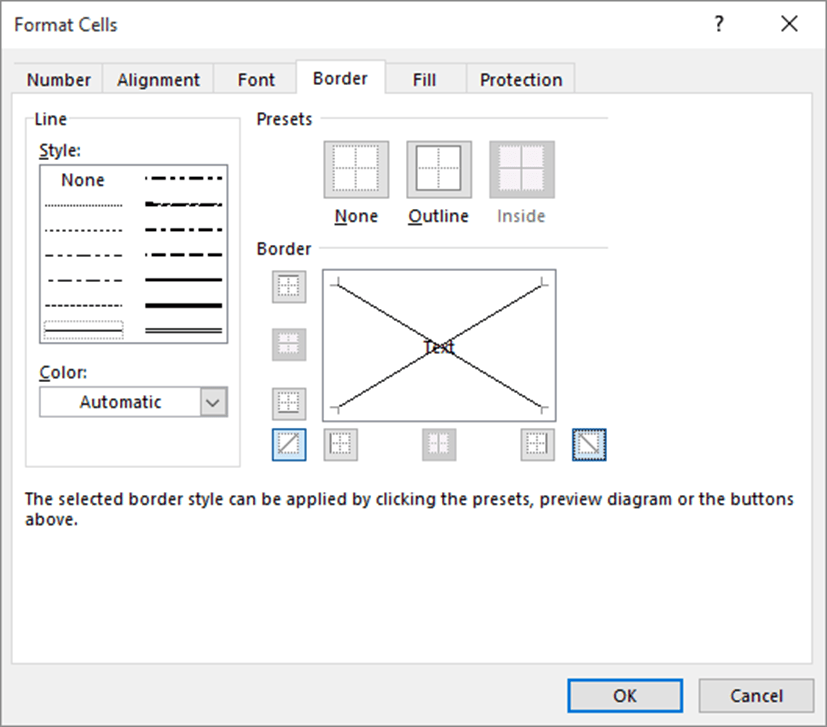
To cross out a cell in Excel, you can use the “Strikethrough” formatting option. Here’s how:
1. Open Excel and select the cell or range of cells you want to cross out.
2. Right-click on the selected cells and choose “Format Cells” from the context menu.
3. In the Format Cells dialog box, go to the Font tab.
4. Under the “Effects” section, check the box next to “Strikethrough”.
5. Click OK to apply the formatting and close the dialog box.
Note: It’s important to mention that this formatting option only visually crosses out the cell content and does not affect any calculations or formulas within the cell.
By using the Strikethrough feature in Excel, you can easily show that a particular cell or range of cells should no longer be considered or included in your calculations. This can be handy in scenarios where you want to highlight outdated information or indicate that certain data is no longer relevant.
Another useful tip is to use conditional formatting to automatically cross out cells based on specific criteria. For example, you can set up a rule to cross out cells that contain a certain value or meet a particular condition. This can be done by going to the Home tab, selecting “Conditional Formatting,” and choosing “New Rule” to define your custom formatting rules.
With these tips, you can efficiently cross out cells in Excel and effectively communicate changes or updates in your data.
Frequent Questions
How do I cross out a cell in Excel?
To cross out a cell in Excel, you can use the “strikethrough” feature. Simply select the cell(s) you want to cross out, then click on the “formatting” options in the toolbar and choose the “strikethrough” option.
Can I undo or remove the cross out effect in a cell in Excel?
Yes, you can remove the cross out effect in a cell in Excel by selecting the cell and clicking on the “Strikethrough” button in the formatting toolbar (Ctrl + 5).
Is it possible to customize the appearance of the cross out effect in Excel cells?
Yes, it’s possible to customize the appearance of the cross out effect in Excel cells by using conditional formatting.
In conclusion, the use of Excel’s cross out cell feature in the realm of technology provides a powerful tool for data analysis and presentation. Whether it’s for highlighting errors, indicating completed tasks, or simply organizing information, this feature enables users to visually communicate important data points in a clear and efficient manner. With its flexibility and ease of use, Excel’s cross out cell feature remains an invaluable asset for tech-savvy individuals seeking to enhance their data management capabilities. Stay ahead of the game by mastering this simple yet impactful technique, and unlock the full potential of your data-driven endeavors.